Evaluate data from Komoot with Elasticsearch and Kibana

In my spare time I like to travel by bike. As a data enthusiast it's no question to track my trips using services such as Komoot. Besides the data analysis methods that these companies provide on their websites or apps, they are always limited in what kind of analysis they provide to their customers. Most of the time it is not enough tough. Having access to the raw data allows to do further analysis and implement highly customized charts.

# Table of content

For convenience this post is divided in five sections:

1. Preconditons
   In this section the necessary tools are explained and installed on your developer machine.
2. Data mining
   In this section the raw data is accessed which will be further analyzed in later steps. No advanced techniques are used for data mining as the focus in this post lies on the next two steps.
3. Data preprocessing
   Using the raw data it's possible to pre-process them in order to simplify the data analysis in the next step. In this step the data will also be imported into the database.
4. Data analysis and visualization
   Custom analysis and charts are implemented in this section.
5. Sumary and outlook
   Having all the data available in Elasticsearch it's possible to do a lot more. This outlook will give a few more ideas what to do next.

Let's start!

# Preconditions

To analyze the data the so called ELK-Stack or Elastic Stack (Elasticsearch, Logstash, Kibana) is used.

An instance of Elasticsearch and Kibana is required to run on the machine in order to analyze the data later on. To simplify the setup process it's best to not install them directly on the development machine but use docker to manage the tools in a virtual environment. By doing so environments are separated, which means that it doesn't matter what operating system your working machine runs - Windows, macOS or Linux - and what versions of tools you have installed. The containers are isolated and describe their own system and dependencies. In case you haven't used docker yet, make sure to install docker first. To get started quickly I have created a dockerized environment that can be used directly.

# clone the Docker Elastic Stack description into the folder named komoot-analysis
git clone https://github.com/dotcs/komoot-elk-jupyter.git

cd komoot-elk-jupyter    # change to this directory
docker-compose up        # spin up the ELK stack and jupyter

docker-compose will spin up a network in which one instance of each, Elasticsearch, Logstash, Kibana and Jupyter, is running. They share the same network configuration so that they can talk to each other.

If everything went fine the following links should work on your developer machine:

• Kibana: http://localhost:5601
• Jupyter: http://localhost:8888

Alright, we've finished the first step in which we spun up a complex development environment that allows for intensive data analysis. Now everything is set up to continue gathering the data. Let's move on!

# Data mining

While Komoot provides an experimental API, it seems impossible to create an application token without participating in some kind of beta program. My issue in the corresponding github project has not been answered yet, so a workaround is necessary to get access to the data.

Fortunately it's easy to call the official API endpoints from the browser when logged in into their web application, because it uses the very same API. For the necessary API call you must be aware of your personal USER_ID. It can be extracted from the link to the profile in the web application, which has the following schema: https://www.komoot.de/user/{USER_ID}. In my case it is 320477127324.

In order to fetch your latest data in JSON format, use the following URL: https://www.komoot.de/api/v007/users/{USER_ID}/tours/. Save the content of this file to jupyter-notebooks/data/komoot.json, it will be needed in the next step.

# Data sample

A single entry does look like this. Note that some information was omitted to save space and it's not used in this blog post anyway.

{
  _embedded: {
    tours: [
      {
        status: "public",
        type: "tour_recorded",
        date: "2017-06-03T14:14:37.000+02:00",
        name: "Runde an der Würm entlang",
        distance: 42980.88913041058,
        duration: 7660,
        sport: "touringbicycle",
        _links: {
          creator: { href: "http://api.komoot.de/v007/users/320477127324/profile_embedded" },
          self: { href: "http://api.komoot.de/v007/tours/17503590?_embedded=" },
          coordinates: { href: "http://api.komoot.de/v007/tours/17503590/coordinates" }
        },
        id: 17503590,
        changed_at: "2017-06-03T15:06:51.000Z",
        kcal_active: 880,
        kcal_resting: 154,
        start_point: {
          lat: 48.795956,
          lng: 8.85,
          alt: 426
        },
        elevation_up: 548.1543636580948,
        elevation_down: 544.0455472560726,
        time_in_motion: 7236,
        map_image: { /* ... */ },
        map_image_preview: { /* ... */ },
        _embedded: {
          creator: { /* ... */ },
          _links: { /* ... */ } },
          display_name: "Fabian Müller"
          }
        }
      },
      /* ... other tour entries ... */
    ]
  }
}

# Data preprocessing

To analyze the data it needs to be imported into Elasticsearch first. To do so I'll preprocess the data using Python with Pandas.

Create a new notebook by opening Jupyter and click on New > Notebook > Python 3.

First all necessary modules need to be imported.

import json
import pandas as pd
from pandas import DataFrame, Series
from elasticsearch import Elasticsearch

Next a connection to Elasticsearch is established.

es = Elasticsearch(hosts=['localhost'], http_auth="elastic:changeme")
es.info()

Output:

{
    "cluster_name": "docker-cluster",
    "cluster_uuid": "Dvit14MhRgiEoTxfIkuzYA",
    "name": "osb6xs4",
    "tagline": "You Know, for Search",
    "version": {
        "build_date": "2017-04-28T17:43:27.229Z",
        "build_hash": "780f8c4",
        "build_snapshot": False,
        "lucene_version": '6.5.0',
        "number": '5.4.0'
    }
}

Now that the notebook and Elasticsearch are connected it's time to read the data in Python.

# Read data into python dictionary.
# Use `data/komoot-sample-data.json` in this call to read the sample data.
with open('data/komoot-sample-data.json') as data_file:
    data = json.load(data_file)
df = DataFrame(data['_embedded']['tours'])

First data is loaded into the data variable, then only the list of tours is loaded into a pandas DataFrame.

Before filling the data into the database it's worth to have a closer look into the data structure. Especially the start point of each tour seems to not match what Elasticsearch can work with. Elasticsearch defines so called geo_points, which are required to have a special format. To make use of geo_points the format needs to be transformed a bit. Let's first tell Elasticsearch that it should expect a geo_point here:

mapping = '''
{
  "mappings": {
    "tour": {
      "properties": {
        "start_point": {
          "type": "geo_point"
        }
      }
    }
  }
}'''
es.indices.create(index='komoot', ignore=400, body=mapping)

This piece of code creates an index called komoot in which it tells Elasticsearch to expect start_point to be of type geo_point. The document type is called tour in the index. It's necessary to transform the data before sending it to Elasticsearch:

df['start_point'] = df['start_point']\
    .map(lambda item: [item['lng'], item['lat']])

This transforms the start_point column from a dictionary into a list with two entries, longitude and latitude of the starting point of the tour.

Next the data can be send to Elasticsearch which will create the rest of the search index automatically based on the types of the input values.

for i, row in df.iterrows():
    res = es.index(index='komoot', doc_type='tour', id=item['id'], body=row.to_json())
    print(row['id'], res['result'])

# output
# 17342318 created
# 17140311 created
# 17069942 created

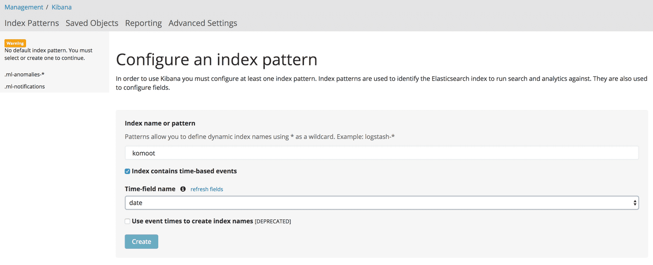
In the next steps Kibana is used to query data and generate some nice plots from it. The remaining thing to do is to tell Kibana that komoot is the preferred index. To do so go to Kibana, log in by using the default username (elastic) and password (changeme) which should bring you right to the Management tab in which a default index must be selected. In this screen use komoot as the index name, check that it contains time-based events and set the time-field name to be date. Click on create to configure the index pattern.

Kibana: Interface to configure an index pattern

# Data analysis and visualization

Now comes the most interesting part - the data analysis. In this section charts will be built using Kibana which accesses Elasticsearch to provide real-time charts. In our case the data is quite sparse compared to server logs, for which Kibana is developed and where you have up to hundreds of logs per second, but nevertheless we will create charts that will change over time, so it's nice to have them encapulated in Kibana. After creating such charts it's only necessary to push new data to Elasticsearch to get them updated. It's as easy as that. Okay, let's see how this works.

We'll create three types of visualizations in this tutorial:

• A tile map of all recorded tours
• A heatmap of distance over time
• A bar chart of time in motion and elevation

Also a Dashboard containing all the previous charts will be created.

# Tile map of all recorded tours

Create a new visualization via Visualize > Plus Icon (Create new visualization) and choose Tile Map. On the next page select komoot as the index. This will create a map with no content yet.

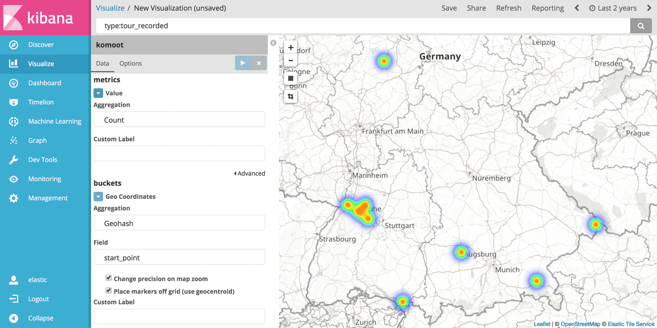
To show a heatmap based on all recorded tours, choose Geo Coordinates as the bucket. This will automatically set up Geohash as the aggregation type and the field start_point since it is the only entry of type geo_point in the schema of the index. Click tab Options and choose Heatmap as the map type. Depending on the data it might be useful to fine-tune the parameters in this tab later on. To only select the recorded tours and ignore the planned ones, type type:tour_recorded into the search bar at the top of the screen. Make sure to choose a proper time span in the upper right corner (e.g. use the last two years or so). I cannot say how often I have forgotten to do so and wondered why there is no data to display. ;-)

Press the primary button ► (Apply Changes) to see your result. You might need to zoom in into the region where your data points are located. Et voilà there it is, enjoy your first heatmap!

Geo-Heatmap of recorded tours

Once you're satisfied with the result save the map by clicking on Save at the top of the screen and choose a proper name, e.g. "Komoot: Geo-Heatmap of recorded tours". This allows to add the chart to a dashboard later on.

# Heatmap of distance over time

Next let's see how well we are performing. I'd like to know how often I went for a ride and how long my rides are.

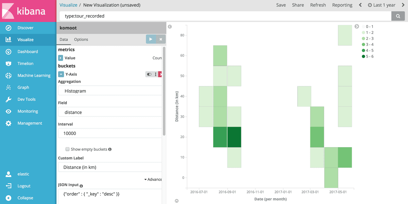
Go to Visualize > Plus Icon (Create new visualization) > Heat Map. Again select komoot as the index, and define a Y-Axis first. Choose Histogram as the aggregation type and choose distance as the field. Define a proper interval, for me 10000 or 10km per bucket worked fine. Click on Advanced and set {"order" : { "_key" : "desc" }} as the JSON input. This tells Kibana that the Histogram should be sorted by the key of each bucket. Click on Add sub-buckets to add a X-Axis and choose Date Histogram as the sub-aggregation type. Set date as the field and Monthly as the interval.

Again set type:tour_recorded into the search bar at the top of the screen to limit the results to the recorded tours.

Heat map: Distance (buckets) over the time (buckets)

Once you're satisfied with the result save the map by clicking on Save at the top of the screen and choose a proper name, e.g. "Komoot: Heatmap distance over time". This allows to add the chart to a dashboard later on.

# Bar chart of time in motion and elevation

Now let's see how the average time in motion varies over time and combine that with the average elevation in a given time interval.

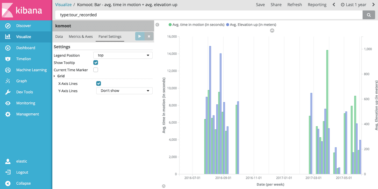
Go to Visualize > Plus Icon (Create new visualization) > Vertical Bar. Select komoot as the index and set the X-Axis to be of type Date Histogram. Choose a Weekly interval. Then define two Y-Axis, where one has aggregation type Average and field time_in_motion. The other one is also of aggregation type Average but has set elevation_up as its field.

Then go to tab Metrics & Axes and add a second Y-Axis. Afterwards in section Metrics set both axis to type normal.

And once again do not forget to set type:tour_recorded in the search bar at the top of the screen to limit the results to the recorded tours.

This gives a nice bar chart that shows the average time in motion as well as the average upwards elevation. Seems like I have climbed a lot more in average in the last year than nowadays. Do I get old? ;-)

Bar chart showing average time in motion and average upwards elevation

# Dashboard

To sum up the visualization part let's create a dashboard. It will be used to display all charts side by side to each other. The main purpose is to interactively explore data. Since all visualizations are connected in the dashboard changing the search query or time interval will update all visualizations at once. Let's get started!

Click on Dashboard > Plus Icon (Create new dashboard) to create a new dashboard. Then click Add at the top of the screen and select the visualizations we have created before. You can re-arrange them as you like, also the size and position can be changed. To save the dashboard click Save on the top of the screen and give it a proper name, e.g. Komoot. I'd recommend to store the time by checking Store time with dashboard. This will update the currently selected time span each time the dashboard is opened.

Custom dashboard with custom visualizations in Kibana

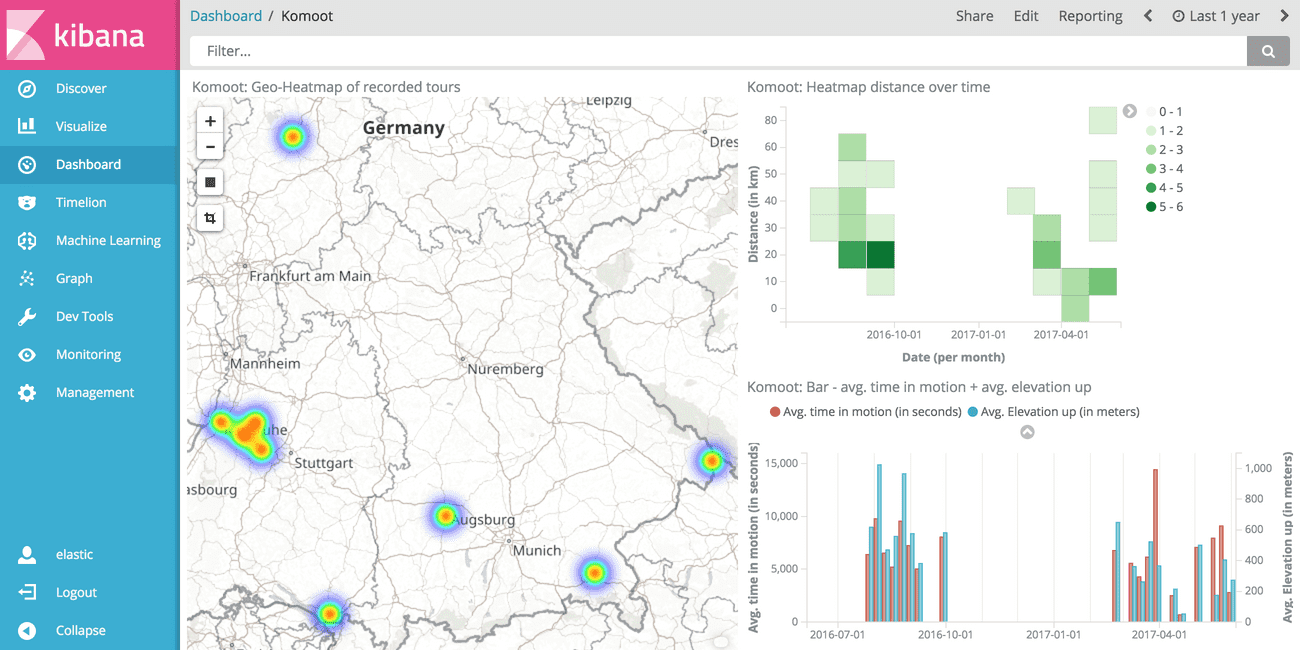
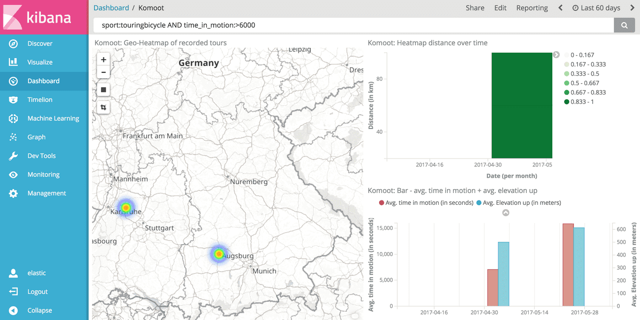
Note that you can use the search query to further reduce the number of results. This will automatically update all charts which is super useful if you have a bunch of charts that you want to keep in sync.

Changing search queries will automatically update the visuals

# Summary and Outlook

Let's recap what we have done on our journey to create a dashboard with customized charts.

We used a dockerized environment to spin up containers which isolate Elasticsearch, Kibana and Jupyter. This technique in itself is very helpful to isolate environments and get rid of any dependency hell issues. I highly recommend to work in dockerized environments as these enviroments can be shared easily, such as I have done it by providing you a git repository that defines all the needed tools.

Data mining has been done by calling an API endpoint by hand and copying the data manually. Although it was simple to do, this is no good solution as it requires to manually log into a website to generate the necessary authentication credentials. I'd like to do better here, which means using the OAuth2 layer of the API, but currently this seems not possible. In case you can use an OAuth layer I'd recommend to do so, because by doing so the data can be requested automatically and therefore the database can be updated regularly with the latest and freshest data available.

For data preprocessing we have used Python and Pandas which I like to work with. Of course other tools are available and there is no need to use the tools I've used. Feel free to use whatever you like to work with. This section also gives a lot of freedom what to do next. Besides using Python only to preprocess data also analytics could be done here. As we have connected Python with the Elasticsearch database, it's easy to do queries here against the database. The elasticsearch module comes with a large API and you should definitively have a look what else it can do. We could also either visualize data directly in Python using matplotlib or other libraries or maybe do some kind of Machine learning. Sky is the limit at this point.

After we've put the data into the database we have analyzed it using Kibana, a powerful frontend for Elasticsearch. We have generated our own visualizations which are easy to create and highly dynamical. We have created a dashboard to group multiple charts and make them dependent on the same query and time interval. This can be a large time saver when digging into the data to gain more and more insights. If you want to show your work to others, note that dashboards can be shared. But note that sharing requires to have the stack running on a server, not only on your local dev machine.

I hope you enjoyed this article. Let me know if you have any questions or remarks.